Back to Top

We are fortunate in DBS surgery that we can acquire large volumes of clinical data to assess our surgical outcomes robustly. Below are some analyses to show what can be done quickly and efficiently (with a little bit of coding). By doing this, I hope it will be easier to make use of these data, either for audit or research purposes. Also, it's also a really nice way to get into Python and see all the potential it has for data analysis (and more). I've used Jupyter Notebook, Plotly, RainCloudPlots, and seaborn for these examples, all of which are awesome.

To get started, just download the data from my Github repository. It uses the terrific Jupyter Notebook so you can literally just click through the examples below. I've set it up to run using the randomised data provided, so the actual results of the analysis shouldn't be interpreted. I've also included a nice example excel file formatted in a way to make data entry straightforward. To analyse your own data, just add it to the spreadsheet. Have fun :)

To start we perform some exploratory data analysis. This first example is a plotmatrix of all outcome variables. It can be used to gauge whether there is any covariance / redundancy between the outcome variables, in which case one may consider removing them from subsequent modelling. You also get a histogram of the data spread along the diagonal.

The next analysis plots the electrode contacts. This uses a violin plot which is really helpful for showing the boxplot, data distribution, and raw data too. Note that the closest contact to the target nucleus is used. I've compared targetting between two different nuclei, as well as accuracy with the overall nucleus and specific motor component.

Now we move on to assessing change in outcomes before and after surgery. Similar to the violin plots above, RainCloudPlots are tremendously useful in not only showing a boxplot but also data distribution and raw data. With this we can assess not only the change in summary statistics but inspect how the raw data may change too.

So far we have assessed the raw data for our outcomes of interest, checked if they are independent, and looked at our electrode accuracy. Next, we may wish to inspect how our outcomes related to electrode placement. Here is a simple linear regression analysis. The distributions for the dependent and independent variables are displayed, as is the regression line with fit and raw data. A lot of information on one simple plot, but it's necessary for accurate analysis visualisation.

Finally, we may wish to assess how multiple variables affect our outcome of interest. Here we use multiple regression to assess how motor outcome is affected by accuracy for different targets.

To say I'm a big Matlab fan would be an understatement. Fortunately, functional neurosurgery affords many opportunities for using Matlab, and in return Matlab can offer some exciting rewards for functional neurosurgery. Here are some examples based off the terrific Lead-DBS toolbox (also written in Matlab).

First, making "Fusion Reports" (post-op assessment of DBS accuracy) is a routine part of DBS clinical practice, both for audit and patient management. Here is a simple way to use some of the interesting data with Lead-DBS - electrode contact distances and 2D locations - to efficiently make a pdf report. It's also a great way to get into using LaTeX. Why not just use another word processor? Using LaTeX makes organising all the images really simple, the whole pipeline works automatically (only a few inputs e.g. patient name are required), and it produces a professional pdf that is also nice and small. To run this, open your Lead-DBS analysis in Matlab then run the script lead_distances_latex.m (select your target inside this script). This generates the text report you then copy into the relevant part of fusionreport_latex.tex file. Here's one I made earlier:


    %LEAD_DISTANCES_LATEX Script to extract data on lead accuracy
    %
    %   Provides data for latex reports.
    %
    %   Usage: define target,      STN, GPI, VIM
    %
    %   Outputs: .mat & .csv file of distances + plots & coords
    %
    %   NB: needs ea.stats open
    %   NNB: set for atlas Distal (medium)
    %
    % Michael Hart, University of British Columbia, August 2020


In a similar mind, it's also good to include location accuracy data in a surgical logbook or database. Try this simple script to do the job:


    %LEAD_LOGBOOK Report on electrode accuracy (e.g. for a surgical logbook)
    %
    %   Usage:  define target,          STN, GPI, VIM
    %           define "in" distance,   distance considered inside the target
    %
    %   Outputs: .mat & .csv file of distances + plots & coords
    %
    %   NB: run from patient directory - needs ea.stats open
    %   NNB: all atlases are Distal (medium)
    %
    % Michael Hart, University of British Columbia, November 2020


Moving on, if you have group data, you may wish to look for trends in accuracy (e.g. Is the second side for implantation more variable in terms of accuracy due to brainshift? Or is their a systematic error with the frame?). This makes a various types of 2D & 3D heatmaps with contour plots to inspect these data more easily.


    %%lead_radar
    %
    % Script for analysing electrode targeting
    %
    % Just set group directory & target below
    %
    % NB: set for distal medium atlas
    % NNB: saves & returns to group directory
    %
    % Michael Hart, University of British Columbia, December 2020


Some centres have a significant volume of single sided implantation (e.g. for tremor). Here is a way to incorporate these into your Lead-DBS workflow (although the most recent version from ~2.5+ should manage this now).


    %LEAD_FLIPPER Duplicates leads for viewing single side results as a group
    %
    %   Usage: subject to duplicate,      absolute path
    %
    %   Outputs: ea_reconstruction.mat in new lead_flipped folder within working directory
    %
    %   NB: set for Medtronic 3389
    %
    %   NNB: code based on discussion here
    %   [https://www.lead-dbs.org/forums/topic/export-code-for-vta-calculation/]
    %
    % Michael Hart, University of British Columbia, November 2020


Multiple different models for VAT (volume of activated tissue) or VTA (volume of tissue activated) analyses are available to help visualise the effects of stimulation. While these vary in some of their parameters and design principles, which is best? And moreover just how do these differences affect the end outcome? Use this simple script to quickly and simply run multiple different VAT analyses. There might not be a 'right' answer (yet!), but at least we can get familiar with the modelling process.


    %MULTI_VAT Compares difference VAT models
    %
    % Makes VATs with multiple (3-4) models
    % Outputs VATs in separate folders
    % Also DICE coefficient confusion matrix
    %
    % nb: works from patient directory
    % nnb: need to run first stimulation in Gui & name it "vat_horn"
    %
    % Michael Hart, University of British Columbia, May 2021


Finally, the group analysis I showed above (in Python) can also be done in Matlab. I'd emphasise that it's not the programming language that makes the difference here, but rather the data and thought that goes into the analysis that counts (although each comes with some pretty neat features).

We can start by analysing the outcomes with plotmatrix & rainclouds.

Then we can move on to analysing electrode accuracy. Here are two styles of plots comparing sides, targets, distances, and volumes of activated tissue (VATs).

Finally, we can compare outcomes with accuracy. Don't forget to correct for multiple comparisons!

Diffusion imaging and tractography have made invaluable contributions to our understanding of the brain in a relatively short time. Fortunately, it's not that difficult to get some basic diffusion imaging on clinical MRI scanners. I wanted to help inspire people to look at these data by showing what can be done and providing the means to do it. Hopefully, this will be a stepping stone to some collaboration between clinical centres, both in terms of code and sequence development. Note that this isn't meant to be a definitive guide to doing DBS with tractography, and the sequences utilised are designed on purpose to be straightforward (and hence mirror what is achievable clinically). Most importantly, I hope it's fun :)

NB: this code wouldn't be where it is without the perpetual inspiration and guidance of Dr Rafael Romero-Garcia ('El Cunado') - muchas gracias!

All the code is available via Github.


            =============================================================================================

            tract_van.sh

            (c) Michael Hart, University of British Columbia, August 2020
            Co-developed with Dr Rafael Romero-Garcia, University of Cambridge

            Function to run tractography on clinical DBS data (e.g. from UBC Functional Neurosurgery Programme)

            Based on the following data: GE scanner, 3 Tesla, 32 Direction DTI protocol

            Example:

            tract_van.sh --T1=mprage.nii.gz --data=diffusion.nii.gz --bvecs=bvecs.txt --bvals=bvals.txt

            Options:

            Mandatory
            --T1            structural (T1) image
            --data          diffusion data (e.g. standard = single B0 as first volume)
            --bvecs         bvecs file
            --bvals         bvals file

            Optional
            --acqparams     acquisition parameters (custom values, for Eddy/TopUp, or leave acqparams.txt in basedir)
            --index         diffusion PE directions (custom values, for Eddy/TopUp, or leave index.txt in basedir)
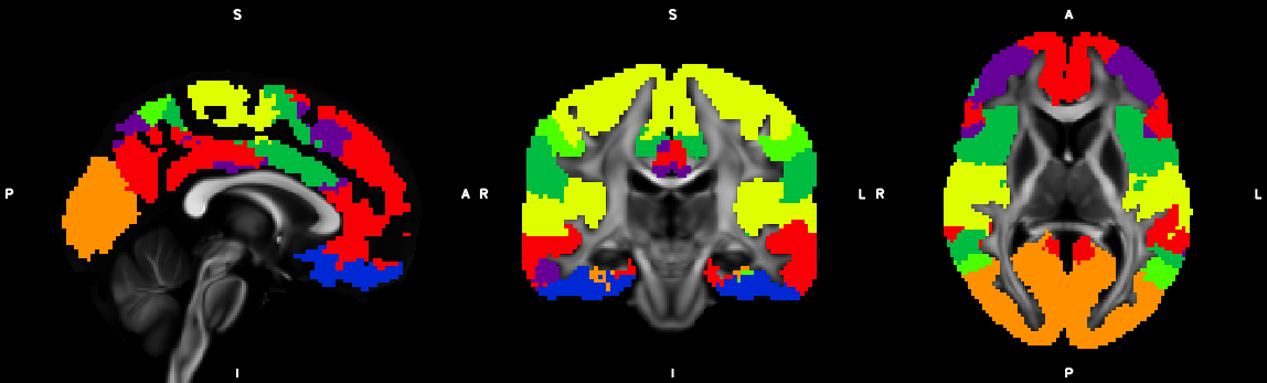
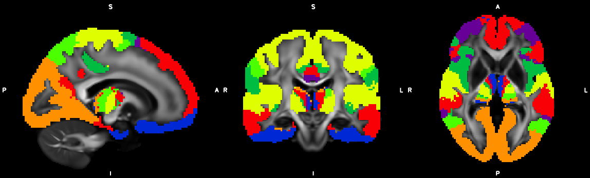
            --segmentation  additional segmentation template (for segmentation: default is Yeo7)
            --parcellation  additional parcellation template (for connectomics: default is AAL90 cortical)
            --nsamples      number of samples for tractography (xtract, segmentation, connectome)
            -d              denoise: runs topup & eddy (see code for default acqparams/index parameters or enter custom as above)
            -p              parallel processing (slurm)*
            -o              overwrite
            -h              show this help
            -v              verbose

            Pipeline
            1.  Baseline quality control
            2.  FSL_anat*
            3.  Freesurfer*
            4.  De-noising with topup & eddy - optional (see code)
            5.  FDT pipeline
            6.  BedPostX*
            7.  Registration
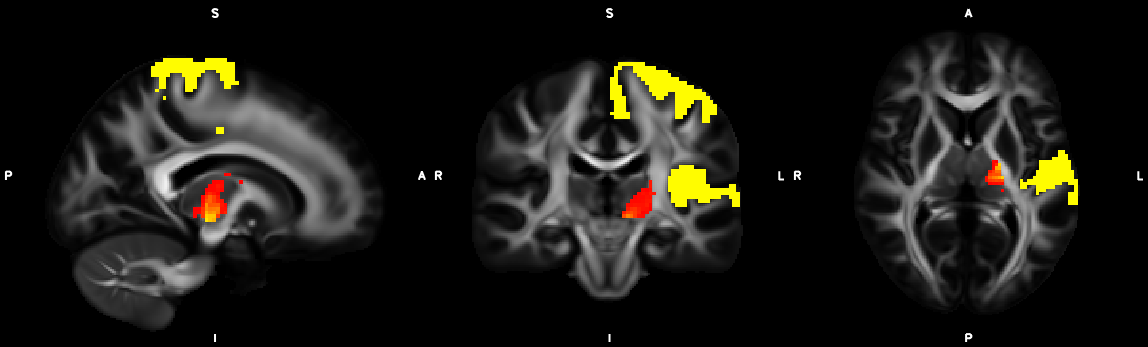
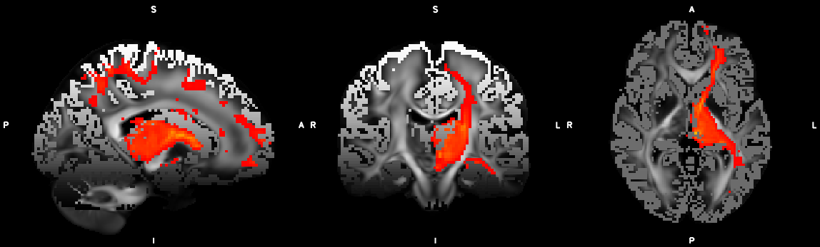
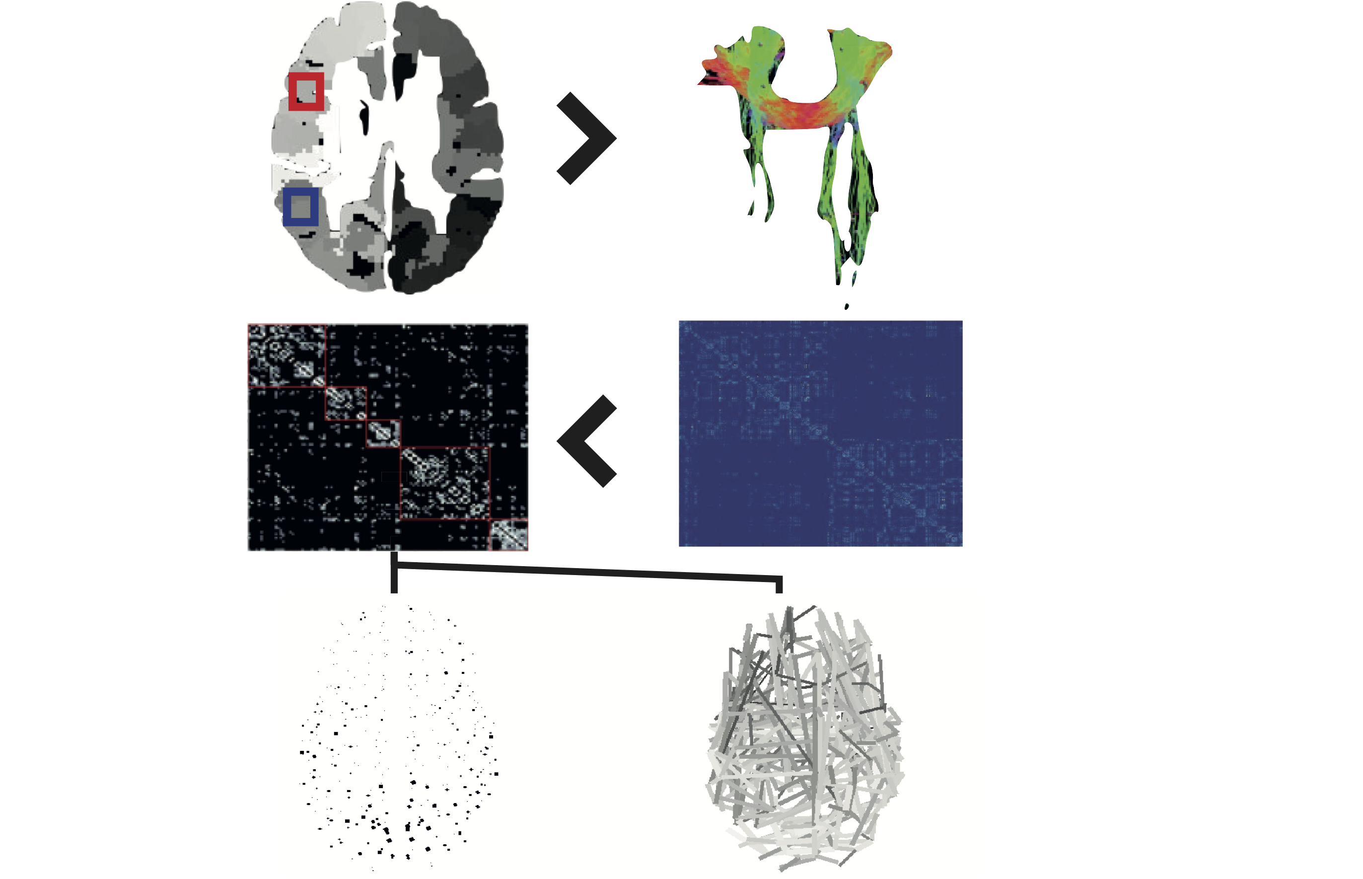
            8.  XTRACT (including custom DBS tracts)
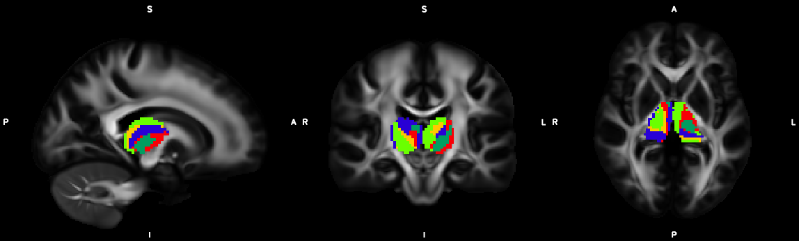
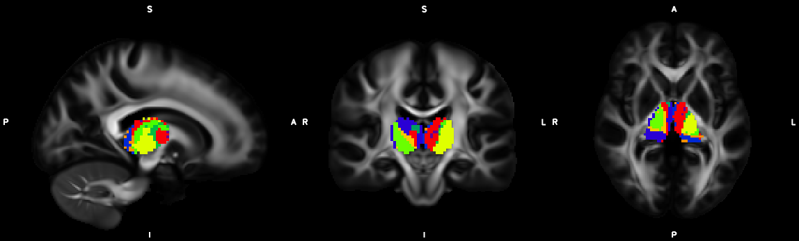
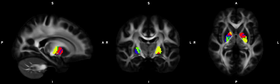
            9.  Segmentation (probtrackx2)
            10. Connectomics (probtrackx2)*

            Version:    1.0

            History:    original

            NB: requires Matlab, Freesurfer, FSL, ANTs, and set path to codedir
            NNB: SGE / GPU acceleration - change eddy, bedpostx, probtrackx2, and XTRACT calls

            =============================================================================================

Set up

Firstly, it's time to set up. Download the code from the github link above and add it to your path e.g. bash_profile. Next there is some standard and freely available neuroimaging software that needs to be installed, plus Matlab if you want to run connectomics. Finally, you need to set the path to codedir in tract_van.sh, and that's it.

In terms of inputs all that are required are a T1 and the diffusion scan with corresponding bvecs and bvals.

Quality Control

Before any analyses, we need to do some quality control. I've made a separate script called tract_QC.sh to help do this. Everything is explained in the usage but basically it produces two outputs: a series of alias calls to help view the pertinent data and analysis steps (e.g. dyads in fsleyes); and a text file of notable values (e.g. SNR, CNR, etcetera). I would also highly recommend the excellent Qoala-T web app for quantitative analysis of FreeSurfer outputs.

Structural

Our analysis begins with the structural image i.e. the T1. This can be an MPRAGE or BRAVO for example, and I've tested at both 1.5T (+/- frame) and 3T. Gadolinium can be given but the enhancement of the dura can make brain extraction and registration more troublesome.

As with any step in neuroimaging it is most important to inspect the raw data. Below is a typical example of a scan we've used (1.5T BRAVO with UCHR & Luminant localiser in-situ).

Our first structural analysis is with FreeSurfer. Below is an example of a typical output. Note that manual refinement and quality control of FreeSurfer outputs is an important topic in itself, for which there is already a large amount already written. Note that I run FreeSurfer QA Tools (which has it's own dependencies) as part of this pipeline.

Now we move on the brain extraction and intensity normalisation. The first method uses the fsl_anat pipeline (beta version) which is a really nice general anatomical processing stream. I use the T1_biascorr_brain as the base for the registrations run later on.

T1_biascorr_brain

I also run the above with ANTs. If this works better for your data it wouldn't be a problem to switch this to be the base for the registrations.

ants_brain

Next we move on to structural segmentation. Here we use FSL FAST to segment grey matter, white matter, and CSF.

fast_segmentation

We also use FSL FIRST to segment selected subcortical nuclei. These masks will be useful later on for the tractography analyses but they are also interesting on their own.

first_segmentation

Our final structural processing is registration. The default I've set up is with FSL (FLIRT & FNIRT) as this is what runs as standard with the Bedpostx GUI and works well on the data I've tested.

diff2standard_fsl

I've also included epi_reg which may work well depending on your data.

epi2standard

Additionally, I've added some ANTs runs for brain extraction (see above), registration (linear & non-linear), and segmentation

diff2standard_ants

Note that all the registrations come with screenshots for ease of comparison and selection of the optimal method for your own data.

Last but not least we do some quality control. Typical measures here include CNR, SNR, and a cost function output for the registration. This is all included in tract_van.sh but its on my to-do list to put it into a stand alone script too.

Diffusion

Now we move on to tractography. I've set this up for Bedpostx & Probtrackx. The main analyses essentially include tractography (both general & DBS specific), subcortical nucleus tractography based segmentation, and connectomics.

As an aside, the analysis has the option to use a clever means of speed up. Here are some brief highlights of this code on lines 674-762:


            #1. Make single slice bedpostx files & submit to cluster
            for ((slice=0; slice<${nSlices}; slice++)); #loop through all of the parts you wish to run in parallel
            do

                ....

                #make a bash file for your command

                #this is the actual commands
                echo 'bedpostx_single_slice.sh ${tempdir}/diffusion ${slice} --nf=3 --fudge=1 --bi=1000 --nj=1250 --se=25 \
                --model=1 --cnonlinear' >> ${tempdir}/diffusion.bedpostX/command_files/command_`printf %04d ${slice}`.sh

                #now submit it to the cluster via Slurm / sbatch
                sbatch --time=02:00:00 ${tempdir}/diffusion.bedpostX/command_files/command_`printf %04d ${slice}`.sh

                ....

            done

            #2. Combines individual file outputs
            #Check if all made: if not, resubmit for longer

            ....

            if [[ "${bedpostFinished}" -ne "${nSlices}" ]] ; #check if the number of outputs matches the number of segments planned to run
            then

                for ((slice=0; slice<${nSlices}; slice++)); #loop through all segments above
                do
                    echo ${slice}
                    if file_doesnt_exist
                    then

                        ....

                        #resubmit bash file above for longer if doesn't exist

                        ....

                    fi
            done

            #3. If all made, run bedpostx_postproc to combine

            #This says it all, just run the same check as in step 2 then it's a one line command

        fi
            

Basically what is happening is the task up is being split into multiple smaller tasks that can be run simultaneously (i.e. in parallel). Then, one can check back in when this is all done, which should hopefully take somewhere around the timing of the overall task divided by the number of segments it has been split into. Finally, the individual tasks are combined. So for example with bedpostx it might take 48 hours without using this approach, but when it's split into 48 separate tasks (slices in this case) it takes just over 1 hour. This is a general technique used in other parts too e.g. for connectomics and a parcellation template >n=100 it really comes into its own. However, it's probably only going to work when using Slurm with many cpu's available. Other means of speeding up would be to use the FSL Sun Grid Engine (SGE) or a GPU.

Many thanks to Dr Rafael Romero-Garcia ('El Cunado') for this incredibly helpful advice and saving years of analysis time.

Tractography

Our first analysis uses the excellent XTRACT programme within FSL to identify 46 canonical tracts using clearly defined and optimised parameters and masks. Here is a video of the overall result:

Below is an image of selected tracts that are more specifically of relevance to DBS. Note that both this image and the movie above were made using xtract_viewer and FSLEYES. Tracts here are anterior commissure, anterior thalamic radiation, corticospinal tract, optic radiation, and superior thalamic radiation. The cursor location is at a left VIM target, but I removed the crosshairs for ease of viewing.

xtract_selected

Note that there are clearly some imperfections here e.g. the registration is off frontally likely due to warping of the diffusion image (which would likely be improved by using multiple B0 volumes with reversed phase encode directions in eddy) and the corticospinal tracts don't show so much angularity at their origin (which would likely be improved by a more HARDI acquisition).

Note also that XTRACT can take quite a while to run with its standard parameters. Ways to speed this up ideally include ideally using a GPU, but one could also submit manual parameters to the function call that will improve the run time (e.g. reducing the number of streamlines).

I've also used XTRACT methods to analyse tracts of particular interest for DBS. These were inspired by the excellent work of Josue Avecillas-Chasin and the Vancouver group. All the masks, parameters, and atlases I've used to create them are available on the Github page.

Below is the denticulorubrothalamic (DRT) tract [seed: cerebellar (dentate) nuclei (Diedrichsen), waypoint: red nucleus contralatral (DISTAL atlas), target: VIM contralateral (DISTAL)].

denticulorubrothalamic tract

Next is the nigrofugal (NF) tract [seed: substantia nigra (DISTAL), target: putaman / caudate / pallidum (DISTAL), exclusion: retrolenticular & anterior limb of the internal capsule (JHU), STN (DISTAL)].

nigrofugal

And finally we have the pallidofugal (PF) tract [seed: pallidum (DISTAL), target: thalamus + substantia nigra (DISTAL), exclusion: retrolenticular & anterior limb of the internal capsule (JHU), putamen + caudate (DISTAL)].

pallidofugal

If one wanted to pursue this line of analysis further there are plenty of avenues one could go down in terms of refining masks and waypoints, for example. However, for this tutorial I've stuck to the fundamentals. Other tracts could be added using this approach too.

Nucleus segmentation

Here the approach is to segment out different parts of specific subcortical nuclei of relevance to deep brain stimulation. The examples I've chosen are the thalamus and pallidum (note this includes both GPi & GPe) from the segmentation by FIRST shown earlier. To begin we perform tractography for all voxels in the selected nucleus (in this case the thalamus).

fdt_paths_thalamus

Next we have a choice of two broad methods for using these data for segmentation. The first is to use a specific cortical target atlas e.g. I've used the Yeo7 fMRI parcellation shown below mainly because it is intuitive, I like the functional-structural link, and I'm just a big fan of this lab's work in general.

Yeo7

Then the number of tracts from each voxel of the nucleus to each region in the cortical target atlas is counted. Here we see those voxels in the thalamus that predominantly connected to the sensorimotor region of the atlas.

Yeo7_sensorimotor

Finally each voxel in the subcortical nucleus is coloured according to the cortical target that it has the most tracts to (using FSL's find_the_biggest). Note it is ever so slightly asymmetrical.

thalamus_findthebiggest

A related approach starts the same way by performing tractography for each voxel in the selected nucleus. However, in this case the target is simply the whole cortex (using a mask of the grey matter from FAST shown earlier), and it is therefore a 'hypothesis free' method (as opposed to using a pre-specified atlas in the approach described above). This is what the method looks like with a cortical mask and thalamic tractography.

omatrix2_thalamus_setup

Each voxel in the specified nucleus now has a specific cortical mask of tract terminations associated with it, stored in a seed_voxel by target_voxel matrix. These cortical masks are then clustered (e.g. using k-means clustering) and each voxel in the selected nucleus identified according to the cluster it falls into. As an aside, k-means is a fascinating analysis in its own right. It's a form of machine learning based clustering when the labels and numbers of categories are known. For further reading there are helpful resources in Matlab and Wikipedia. Note that this step has a separate call to Matlab and requires the numbers of clusters to be specified. Here is an example of the final result.

kmeans_thalamus

Finally here is a comparison of both approaches: k-means on the right brain and biggest segmentation on the left brain.

thalamic_segmentation_2methods

I've also done this approach with the pallidum: again k-means on the right brain and biggest segmentation on the left brain.

pallidal_segmentation_2methods

Other types of segmentation approaches could involve clustering which allows for overlapping regions and varying thresholds.

In general this type of analysis is an excellent method of quality control and getting familiar with the data by following the seminal work of Behren's et al. If you are thinking of pursuing this line of tractography analysis in greater depth, here is a nice starting point to highlight some of the considerations involved.

Connectome

Our final analysis is connectomics. These methods essentially look to create a 'wiring diagram' of the whole brain. In brief, one starts by splitting the brain up into different segments (known as parcels) using a parcellation template. I've used the AAL90 as default as it's well known, anatomical, and in terms of resolution it's on the lower side (which makes some steps a bit easier / quicker). This is a nice place to start, but one may wish to explore different parcellation templates too. After this, tractography is run from each brain segment, and the number of tracts that reach any of the other parcels are counted. This is repeated for all parcels and the data entered in a connectivity matrix. Here each row and column is a different parcel (it's symmetrical), the corresponding interfaces between each row and line (the entries in the matrix) are the number of connections (or now) between them. Once this is computed one can perform a variety of matrix operations / graph theory analyses on it. Finally, one can choose to visualise this analysis in a variety of ways, with or without co-ordinates. I've chosen to look at the nodes (on the left), with more highly connected ones being larger and darker (corresponding to hubs), and edges (on the right, stronger connections being thicker and darker). Below is a brief summary of these methods.

NB: depending on the size of your parcellation template this can take some time. I used the Slurm / parallel speed-up described earlier (see under bedpostx / tractography), so tractography from each parcel is a separate (and very small) job with all parcels run in parallel then combined at the end to form the connectivity matrix. Acceleration with a SGE or ideally a GPU would be ideal, but I think for very large templates this current method may even be faster (assuming you have enough CPU's available).

connectome_methods

Here we move from Bash and the terminal to Matlab. The code for this is in a separate folder of my Github. First lets see the help header in Matlab:


            %% Script for connectome analysis with tractography data
            %
            % Dependencies:     BCT 2019_03_03, contest, versatility, matlab_bgl, powerlaws_full, schemaball, BrainNetViewer
            %
            % Inputs:           data.txt,   connectivity streamlines matrix
            %                   xyz.txt,    parcellation template co-ordinates
            %
            % Outputs:          graph theory measures & visualisations
            %
            % Version: 1.0
            %
            % Includes
            %
            % A: Quality control

            % A1. Load data
            % A2. Basic definitions
            % A3. Connectivity checks
            % A4. Generation of comparison graphs
            %
            % B:  Network characterisation
            %
            % B1. Modularity & Versatility
            % B2. Graph theory measures
            % B3. Normalise measures
            % B4. Measures statistics
            % B5. Symmetry
            % B6. Measures plotmatrix
            % B7. Cost function analysis
            % B8. Small world analysis
            % B9. Degree distribution fitting
            %
            % C:  Advanced network topology
            %
            % C1. Hubs
            % C2. Rich clubs
            % C3. Edge categories
            % C4. Percolation
            %
            % D:  Binary [selected analyses]
            %
            % D1: Measures
            % D2: Clustering
            % D3: Path length
            % D4: Symmetry
            % D5: Hubs
            % D6: Rich club
            %
            % E: Visualisation
            %
            % E1: Basic
            % E2: Edge cost
            % E3: Spheres
            % E4: Growing
            % E5: Rich club
            % E6: Modules
            % E7: 3D
            % E8: Rotating
            % E9: Gephi
            % E10:Neuromarvl
            % E11:Circular (Schemaball)
            % E12:BrainNet

            % Michael Hart, University of British Columbia, February 2021


The actual connectivity matrix is already computed as part of tract_van.sh so we start by loading this up in Matlab together with the parcellation template co-ordinates. To do this you just need to enter the patient path in section A1.


            %% A1. Load data

            %This should be the only part required to be set manually

            %Directory
            directory = '/path_to_my_data';

            %Patient ID
            patientID = 'my_patient_ID';

            %Template name
            template = 'AAL90';


Like tract_van.sh, there are also some dependencies to set up on your path in Matlab.

Early on lets do a quick visualisation. This serves as a good 'sanity check' to make sure our data is good and its processing has been done well. For instance, I had some weird asymmetrical results when I first did this. It turned out my parcellation template wasn't in diffusion space for the network tractography in probtrackx because I hadn't entered the transformations, and this hadn't been flagged as an error during that part of the analysis. The actual matrix looked ok, but it was this visualisation that highlighted it best.

connectome_full

The above is at 30% cost with 90 cortical parcels (AAL) and you can see it's starting to be a little crowded already. To get a better idea of individual features in a network we can create a movie of how the nodes & links load up in order of their weight.

Now we move on to visualising some more advanced network features. Here is a rich club, defined on the basis of disproportionately greater connectivity between hubs defined on consensus criteria, as well as edges that are either entirely within the rich club, feed into it, or purely local and outwith it.

rich_club

After that we move on to defining communities and module partition. There is a bit of work earlier on how to objectively define a reasonable gamma parameter. Here we have a 10 module decomposition and curiously some modules appear to have a contralateral homolog (e.g. 1:9, 2:3, 4:8). In addition 7 appears to be visual/occipital, 6 frontal, while 10 might possibly be noise.

modules

Next up we do some visualisation in 3D. We can rotate this and save it as a movie too, or you can simply spin round the network by hand. This is quite a nice way to explore the network and query any specific connections. A super nice way to do this is to use the excellent package Meshlab (see my 3D printing code on Github for how to transform a connectome to a suitable mesh file using python).

And finally we've got the obligatory BrainNet images because they still just look so good. I've set up custom parameters here which I feel work well, and are included in the Github download (nodestyle & edgestyle).

brainnet

And that's all for now folks. Hope that's been interesting. It would be interesting to know which direction people are most interested in going next e.g. sequence development, de-noising, speed-up, specific tracts, or integrating the pipeline into clinical practice.

NB: this code is to be enjoyed. All comments are welcome, but please see the individual licenses, and note that unfortunately I don't have the resources to offer follow-up support (sorry).